Time Trains#

As demonstrated in earlier posts in the tutorial, pyquickbench can be useful to measure the wall time of python functions. More often than not however, it can be useful to have a more precise idea of where CPU cycles are spent. This is the raison d’être of pyquickbench.TimeTrain. As shown in the following few lines, using a pyquickbench.TimeTrain is extremely simple: simply call the pyquickbench.TimeTrain.toc() method between snippets of code you want to time and pyquickbench takes care of the rest!

import time
import pyquickbench

TT = pyquickbench.TimeTrain()

time.sleep(0.01)
TT.toc()

time.sleep(0.02)
TT.toc()

time.sleep(0.03)
TT.toc()

time.sleep(0.04)
TT.toc()

time.sleep(0.01)
TT.toc()

print(TT)

TimeTrain results:

01005455 s at file 10-TimeTrains.py line 49
02003816 s at file 10-TimeTrains.py line 52
03004684 s at file 10-TimeTrains.py line 55
04003194 s at file 10-TimeTrains.py line 58
01006837 s at file 10-TimeTrains.py line 61

Total: 0.11023987 s

Individual calls to pyquickbench.TimeTrain.toc() can be named.

TT = pyquickbench.TimeTrain()

for i in range(3):
    time.sleep(0.01)
    TT.toc("repeated")

for i in range(3):
    time.sleep(0.01)
    TT.toc(f"unique {i+1}")

print(TT)

TimeTrain results:

repeated : 0.01006465 s at file 10-TimeTrains.py line 73
repeated : 0.01006365 s at file 10-TimeTrains.py line 73
repeated : 0.01006117 s at file 10-TimeTrains.py line 73
unique 1 : 0.01007218 s at file 10-TimeTrains.py line 77
unique 2 : 0.01006285 s at file 10-TimeTrains.py line 77
unique 3 : 0.01006304 s at file 10-TimeTrains.py line 77

Total: 0.06038754 s

Timing measurements relative to identical names can be reduced using any reduction method in pyquickbench.all_reductions.

TT = pyquickbench.TimeTrain(
    names_reduction = 'sum',
)

for i in range(3):
    time.sleep(0.01)
    TT.toc("repeated")

for i in range(3):
    time.sleep(0.01)
    TT.toc(f"unique {i+1}")

print(TT)

/home/gfo/pyquickbench/pyquickbench/_time_train.py:113: UserWarning: include_locs and names_reduction were both enabled. Only the first location will be displayed for every name.
  warnings.warn("include_locs and names_reduction were both enabled. Only the first location will be displayed for every name.")
TimeTrain results:
Reduction: sum

repeated : 0.03018809 s at file 10-TimeTrains.py line 90
unique 1 : 0.01007752 s at file 10-TimeTrains.py line 94
unique 2 : 0.01007652 s at file 10-TimeTrains.py line 94
unique 3 : 0.01006756 s at file 10-TimeTrains.py line 94

Total: 0.06040969 s

Relative measured times can be reported using the keyword relative_timings.

TT = pyquickbench.TimeTrain(
    names_reduction = 'avg',
    relative_timings = True,
)

for i in range(3):
    time.sleep(0.01)
    TT.toc("repeated")

for i in range(3):
    time.sleep(0.01)
    TT.toc(f"unique {i+1}")

print(TT)

/home/gfo/pyquickbench/pyquickbench/_time_train.py:119: UserWarning: Reduction avg combined with "relative_timings = True" will lead to reported timings not adding up to 100%.
  warnings.warn(f"Reduction {self.names_reduction_key} combined with \"relative_timings = True\" will lead to reported timings not adding up to 100%.")
TimeTrain results:
Reduction: avg

repeated : 16.66770650 % at file 10-TimeTrains.py line 108
unique 1 : 16.66453319 % at file 10-TimeTrains.py line 112
unique 2 : 16.66254677 % at file 10-TimeTrains.py line 112
unique 3 : 16.66980052 % at file 10-TimeTrains.py line 112

Total: 0.06041013 s

Reductions make locations ill-defined, which is why pyquickbench.TimeTrain is issuing a warning. Another good reason to disable location recording is that the corresponding call to inspect.stack() can be non-negligible (around 0.01s on a generic laptop computer). Displaying locations can be disabled like so:

TT = pyquickbench.TimeTrain(
    names_reduction = 'sum',
    include_locs = False,
)

for i in range(3):
    time.sleep(0.01)
    TT.toc("repeated")

for i in range(3):
    time.sleep(0.01)
    TT.toc(f"unique {i+1}")

print(TT)

TimeTrain results:
Reduction: sum

repeated : 0.03020864 s
unique 1 : 0.01009330 s
unique 2 : 0.01006893 s
unique 3 : 0.01006521 s

Total: 0.06043607 s

TimeTrains can also time calls to a function. The function pyquickbench.TimeTrain.tictoc() will instrument a given function to record its execution time. The most starightforward is to use pyquickbench.TimeTrain.tictoc() with a decorator syntax:

TT = pyquickbench.TimeTrain()

@TT.tictoc
def wait_a_bit():
    time.sleep(0.01)

@TT.tictoc
def wait_more():
    time.sleep(0.01)


wait_a_bit()
wait_more()

print(TT)

TimeTrain results:

wait_a_bit : 0.01007944 s at file 10-TimeTrains.py line 151
wait_more  : 0.01007003 s at file 10-TimeTrains.py line 152

Total: 0.02014947 s

Using pyquickbench.TimeTrain.tictoc() with a regular wrapping syntax might lead to surprizing results:

TT = pyquickbench.TimeTrain()

def wait_unrecorded():
    time.sleep(0.01)

wait_recorded = TT.tictoc(wait_unrecorded)

wait_unrecorded()
wait_recorded()

print(TT)

TimeTrain results:

wait_unrecorded : 0.01007392 s at file 10-TimeTrains.py line 167

Total: 0.01007392 s

This behavior is to be expected because under the hood, pyquickbench.TimeTrain.tictoc() uses the __name__ attribute of the wrapped function.

print(f'{wait_recorded.__name__ = }')

wait_recorded.__name__ = 'wait_unrecorded'

Overriding the __name__ of the wrapped function gives the expected result:

TT = pyquickbench.TimeTrain()

def wait_unrecorded():
    time.sleep(0.01)

wait_recorded = TT.tictoc(wait_unrecorded)
wait_recorded.__name__ = 'wait_recorded'

wait_unrecorded()
wait_recorded()

print(TT)

TimeTrain results:

wait_recorded : 0.01006476 s at file 10-TimeTrains.py line 188

Total: 0.01006476 s

More simply, you can set a custom name with the following syntax:

TT = pyquickbench.TimeTrain()

def wait_unrecorded():
    time.sleep(0.01)

wait_recorded = TT.tictoc(wait_unrecorded, name = "my_custom_name")

wait_unrecorded()
wait_recorded()

print(TT)

TimeTrain results:

my_custom_name : 0.01006429 s at file 10-TimeTrains.py line 202

Total: 0.01006429 s

By default, a pyquickbench.TimeTrain will not show timings occuring in between decorated function. This behavior can be overriden setting the ignore_names argument to an empty iterator:

TT = pyquickbench.TimeTrain(ignore_names = [])

def wait_unrecorded():
    time.sleep(0.01)

@TT.tictoc
def wait_recorded():
    time.sleep(0.02)

wait_unrecorded()
wait_recorded()

print(TT)

TimeTrain results:

pyquickbench_sync : 0.01009569 s at file 10-TimeTrains.py line 219
wait_recorded     : 0.02007292 s at file 10-TimeTrains.py line 219

Total: 0.03016861 s

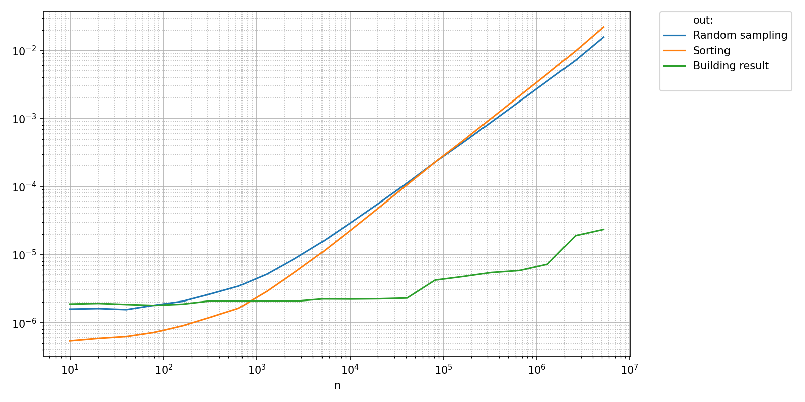
Let’s revisit the benchmark in Vector outputs and measure the execution time of different parts of the function uniform_quantiles using pyquickbench.TimeTrain.

def uniform_quantiles(n, m):

    TT = pyquickbench.TimeTrain(
        include_locs = False,
    )

    vec = np.random.random((n+1))
    TT.toc("Random sampling")

    vec.sort()
    TT.toc("Sorting")

    res = np.array([abs(vec[(n // m)*i]) for i in range(m+1)])
    TT.toc("Building result")

    return TT

This function can be divided up into three main parts:

A random sampling phase, where data is generated. This part is expected to scale as \(\mathcal{O}(n)\).
A sorting phase where the random vector is sorted in-place. This part is expected to scale as \(\mathcal{O}(n\log(n))\), and thus be dominant for large \(n\).
A last phase where estimated quantiles are built and returned. This phase is expected to scale as \(\mathcal{O}(1)\) and be negligible for large \(n\).

m = 10
uniform_decile = functools.partial(uniform_quantiles, m=m)
uniform_decile.__name__ = "uniform_decile"

all_funs = [
    uniform_decile   ,
]

n_bench = 20
all_sizes = [m * 2**n for n in range(n_bench)]

n_repeat = 100

plot_intent = {
    pyquickbench.default_ax_name : "points"         ,
    pyquickbench.out_ax_name : "curve_color"        ,
}

pyquickbench.run_benchmark(
    all_sizes                       ,
    all_funs                        ,
    n_repeat = n_repeat             ,
    mode = "vector_output"          ,
    StopOnExcept = True             ,
    plot_intent = plot_intent       ,
    show = True                     ,
)

Gallery generated by Sphinx-Gallery

Time Trains#

This Page