Plotting transformed values

Let’s expand on the benchmark exposed in Plotting scalar values. The benchmark consists in understanding the convergence behavior of the following ODE integrators provided by scipy.

method_names = [
    "RK45"  ,
    "RK23"  ,
    "DOP853",
    "Radau" ,
]

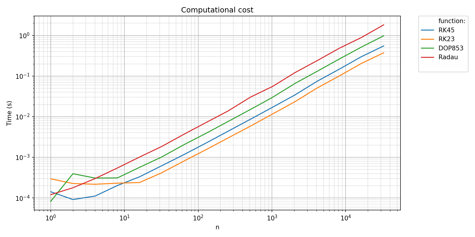
Let’s focus on timings first.

timings_filename = os.path.join(bench_folder,basename_bench_filename+'_timings.npz')
timings_results = pyquickbench.run_benchmark(
    all_nint                                    ,
    bench                                       ,
    filename = timings_filename                 ,
)

pyquickbench.plot_benchmark(
    timings_results                 ,
    all_nint                        ,
    bench                           ,
    show = True                     ,
    title = 'Computational cost'    ,
)

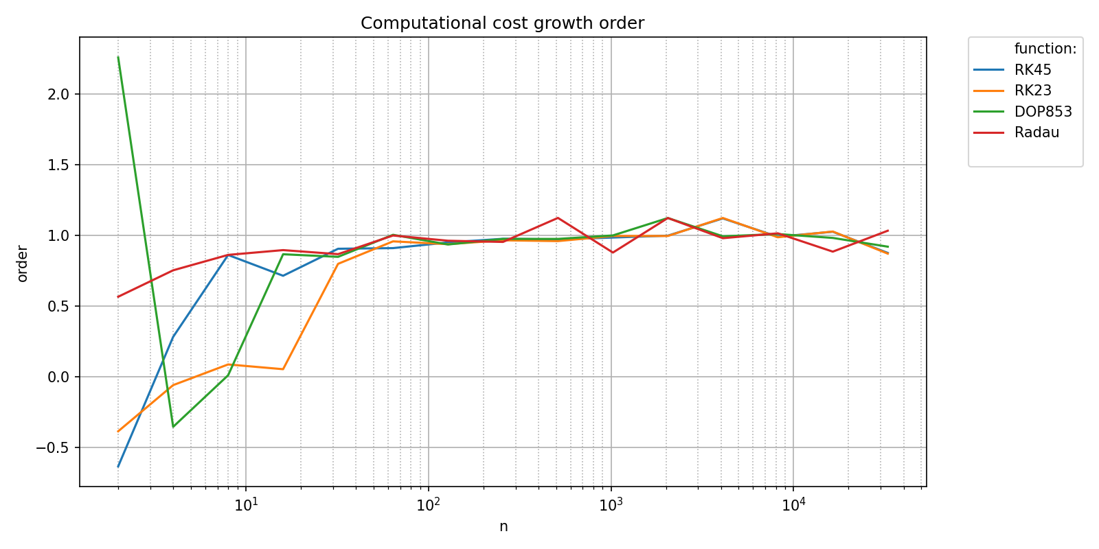
We can check that the integrations algorithms provided by scipy scale linearly with respect to the number of integrations steps with the transform argument set to "pol_growth_order":

pyquickbench.plot_benchmark(
    timings_results                             ,
    all_nint                                    ,
    bench                                       ,
    logx_plot = True                            ,
    title = "Computational cost growth order"   ,
    transform = "pol_growth_order"              ,
    show = True                                 ,
)

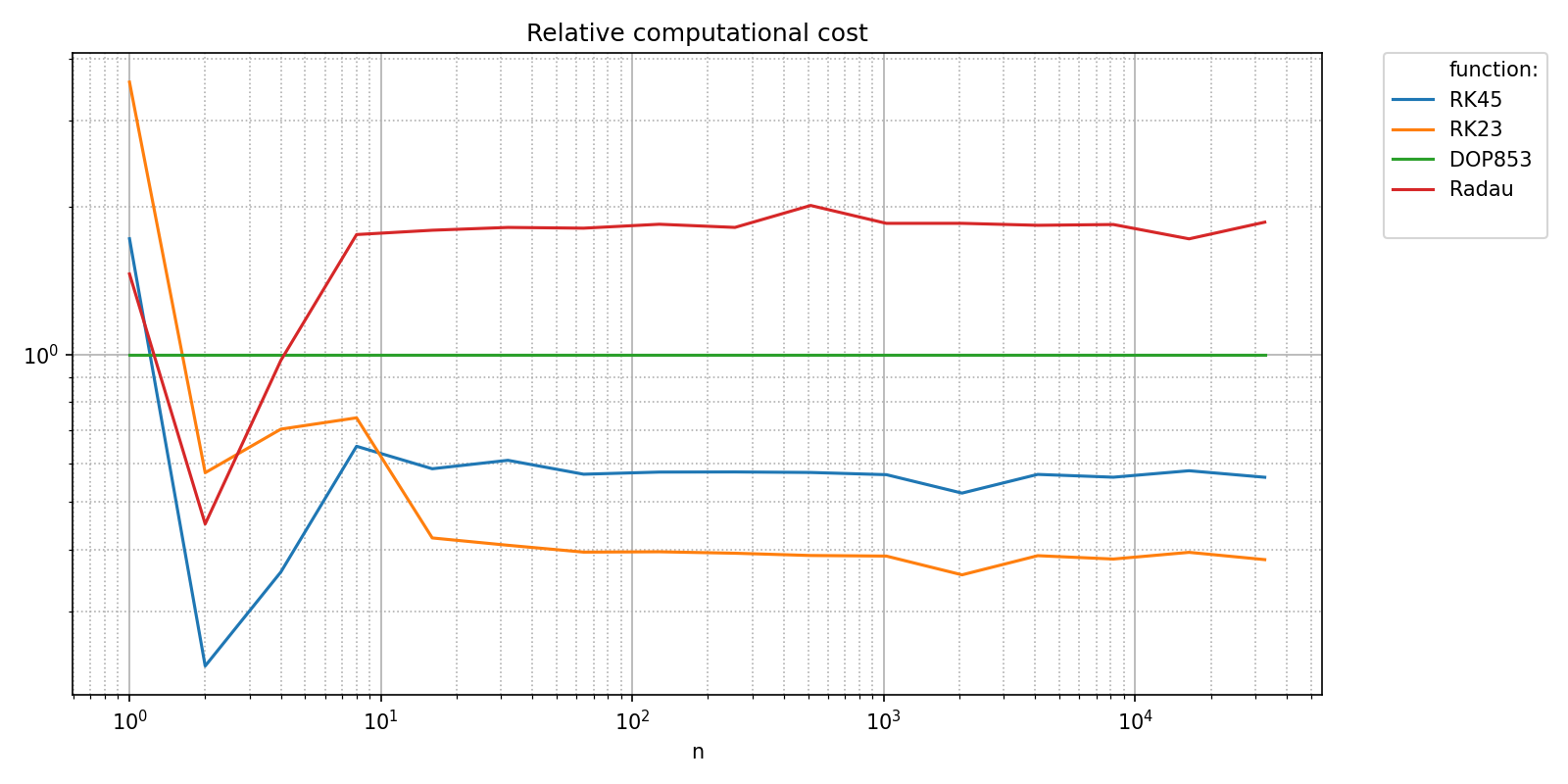
Since all the functions in the benchmark have the same asymptotic behavior, it makes sense to compare then against each other. Let’s pick a reference method, for instance “DOP853” and plot all timings relative to this reference. This is achieved with the relative_to_val argument.

relative_to_val = {pyquickbench.fun_ax_name: "DOP853"}

pyquickbench.plot_benchmark(
    timings_results                         ,
    all_nint                                ,
    bench                                   ,
    logx_plot = True                        ,
    title = "Relative computational cost"   ,
    relative_to_val = relative_to_val       ,
    show = True                             ,
)

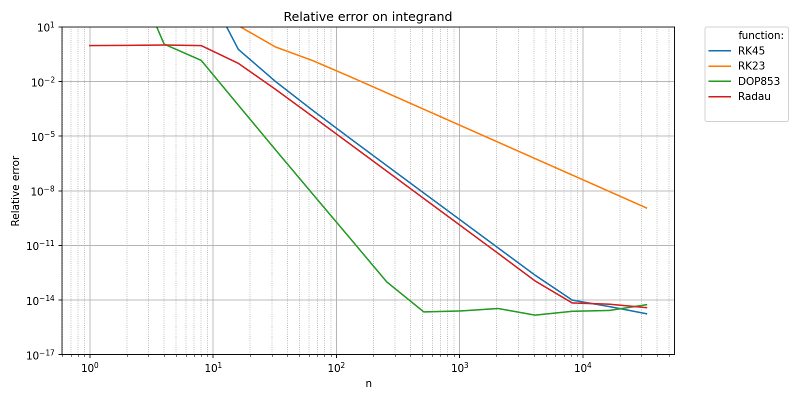
Let’s focus on accuracy measurements now.

plot_ylim = [1e-17, 1e1]
scalar_filename = os.path.join(bench_folder,basename_bench_filename+'_error.npz')
bench_results = pyquickbench.run_benchmark(
    all_nint                                ,
    bench                                   ,
    mode = "scalar_output"                  ,
    filename = scalar_filename              ,
)

pyquickbench.plot_benchmark(
    bench_results                           ,
    all_nint                                ,
    bench                                   ,
    mode = "scalar_output"                  ,
    plot_ylim = plot_ylim                   ,
    title = 'Relative error on integrand'   ,
    ylabel = "Relative error"               ,
    show = True                             ,
)

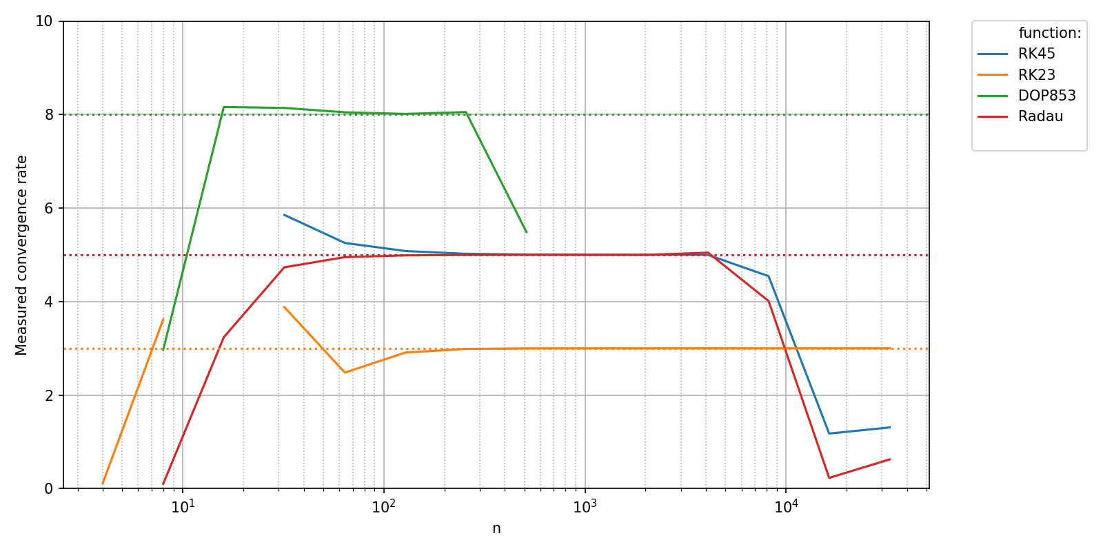
A natural question when assessing accuracy is to ask whether the measured convergence rates of the numerical methods match their theoretical convergence rates. This post-processing can be performed automatically by pyquickbench.run_benchmark() if the argument transform is set to "pol_cvgence_order".

plot_ylim = [0, 10]

pyquickbench.plot_benchmark(
    bench_results                           ,
    all_nint                                ,
    bench                                   ,
    mode = "scalar_output"                  ,
    plot_ylim = plot_ylim                   ,
    ylabel = "Measured convergence rate"    ,
    logx_plot = True                        ,
    transform = "pol_cvgence_order"         ,
    show = True                             ,
)

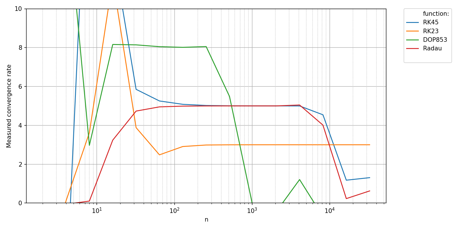
The pre and post convergence behavior of the numerical algorithms really clutters the plots. In this case, a clearer plot is obtained if the argument clip_vals is set to True.

pyquickbench.plot_benchmark(
    bench_results                           ,
    all_nint                                ,
    bench                                   ,
    mode = "scalar_output"                  ,
    plot_ylim = plot_ylim                   ,
    ylabel = "Measured convergence rate"    ,
    logx_plot = True                        ,
    transform = "pol_cvgence_order"         ,
    clip_vals = True                        ,
    show = True                             ,
)

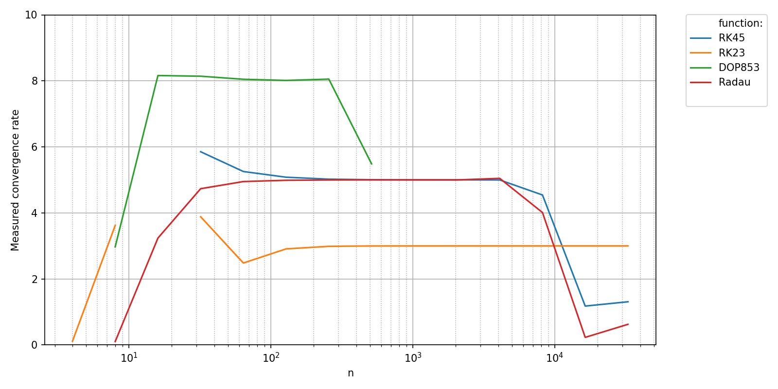
The measured values can now be compared to the theoretical convergence rates of the different methods. In order to plot your own data to the figure, you can handle the matplotlib.figure.Figure and matplotlib.axes.Axes objects yourself, And decouple the calls to pyquickbench.run_benchmark() and pyquickbench.plot_benchmark() as shown here.

th_cvg_rate = {
    "RK45"  : 5,
    "RK23"  : 3,
    "DOP853": 8,
    "Radau" : 5,
}

fig, ax = pyquickbench.plot_benchmark(
    bench_results                           ,
    all_nint                                ,
    bench                                   ,
    mode = "scalar_output"                  ,
    show = False                            ,
    plot_ylim = plot_ylim                   ,
    ylabel = "Measured convergence rate"    ,
    logx_plot = True                        ,
    transform = "pol_cvgence_order"         ,
    clip_vals = True                        ,
)

xlim = ax[0,0].get_xlim()
for name in bench:

    th_order = th_cvg_rate[name]
    ax[0,0].plot(xlim, [th_order, th_order], linestyle='dotted')

ax[0,0].set_xlim(xlim)
plt.tight_layout()
plt.show()