Vector outputs

Pyquickbench can also be used to benchmark functions that return multiple values. This capability corresponds to mode = "vector_output" in pyquickbench. The following benchmark measures the convergence of quantile estimatores of a uniform random variable towards their theoretical values. Let us first observe how the values of the naive quantile estimator as returned by uniform_quantiles evolve with increasing number of simulated random variables:

import pyquickbench

def uniform_quantiles(n,m):

    vec = np.random.random((n+1))
    vec.sort()

    return np.array([abs(vec[(n // m)*i]) for i in range(m+1)])

m = 10
uniform_decile = functools.partial(uniform_quantiles, m=m)
uniform_decile.__name__ = "uniform_decile"

all_funs = [
    uniform_decile   ,
]

n_bench = 10
all_sizes = [m * 2**n for n in range(n_bench)]

n_repeat = 100

all_values = pyquickbench.run_benchmark(
    all_sizes                   ,
    all_funs                    ,
    n_repeat = n_repeat         ,
    mode = "vector_output"      ,
    StopOnExcept = True         ,
    pooltype = 'process'        ,
)

plot_intent = {
    pyquickbench.default_ax_name : "points"         ,
    pyquickbench.repeat_ax_name : "same"            ,
    pyquickbench.out_ax_name : "curve_color"        ,
}

pyquickbench.plot_benchmark(
    all_values                      ,
    all_sizes                       ,
    all_funs                        ,
    plot_intent = plot_intent       ,
    show = True                     ,
    logy_plot = False               ,
    plot_ylim = (0.,1.)             ,
    alpha = 50./255                 ,
    ylabel = "Quantile estimator"   ,
)

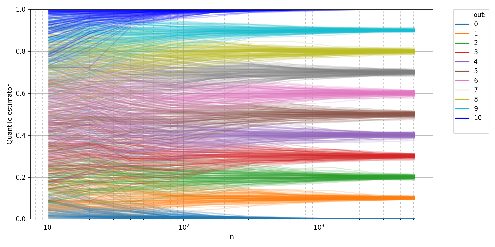
While the above plot hints at a convergence towards specific values, we can be a bit more precise and plot the actual convergence error.

def uniform_quantiles_error(n,m):

    vec = np.random.random((n+1))
    vec.sort()

    return np.array([abs(vec[(n // m)*i] - i / m) for i in range(m+1)])

uniform_decile_error = functools.partial(uniform_quantiles_error, m=m)
uniform_decile_error.__name__ = "uniform_decile_error"

all_funs = [
    uniform_decile_error   ,
]

n_repeat = 10000

all_errors = pyquickbench.run_benchmark(
    all_sizes                   ,
    all_funs                    ,
    n_repeat = n_repeat         ,
    mode = "vector_output"      ,
    StopOnExcept = True         ,
    pooltype = 'process'        ,

)

plot_intent = {
    pyquickbench.default_ax_name : "points"         ,
    pyquickbench.fun_ax_name : "curve_color"        ,
    pyquickbench.repeat_ax_name : "reduction_median",
    pyquickbench.out_ax_name : "curve_color"        ,
}

pyquickbench.plot_benchmark(
    all_errors                      ,
    all_sizes                       ,
    all_funs                        ,
    plot_intent = plot_intent       ,
    show = True                     ,
    ylabel = "Estimator error"      ,

)

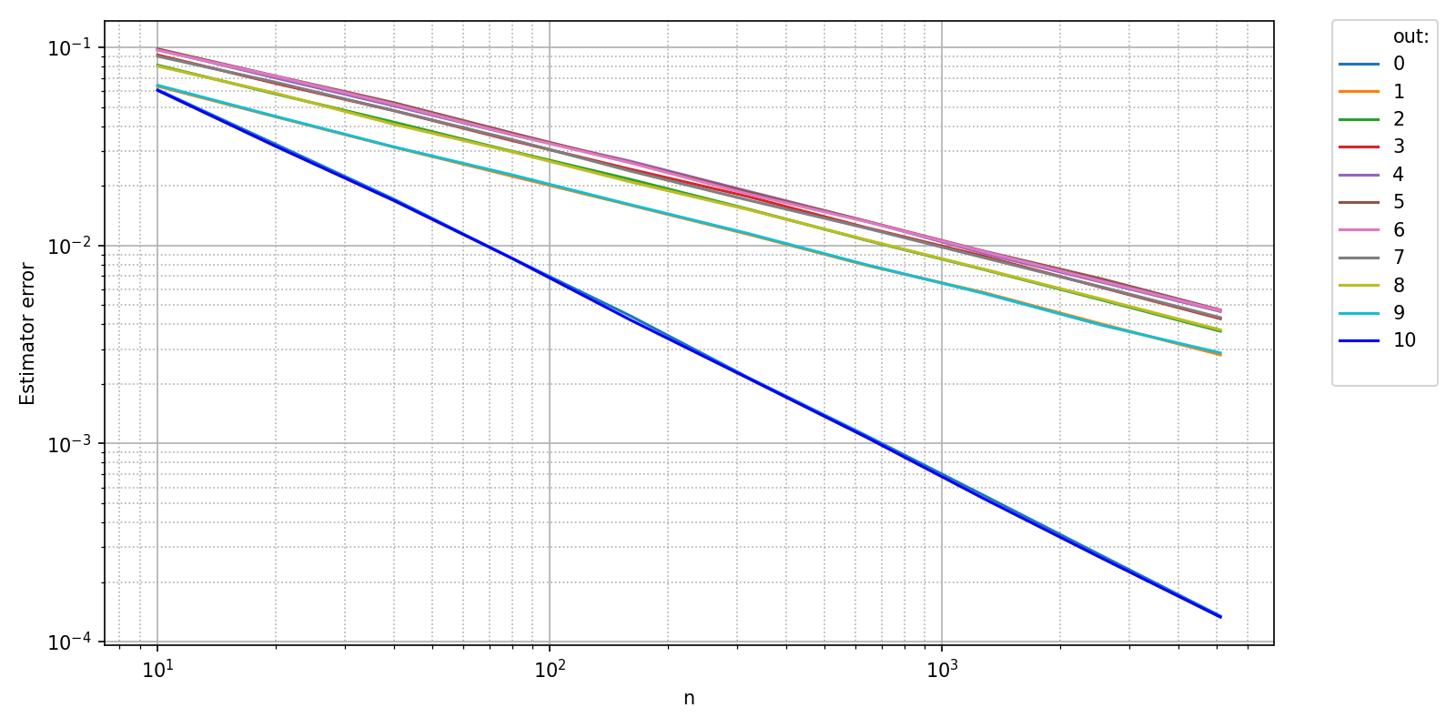
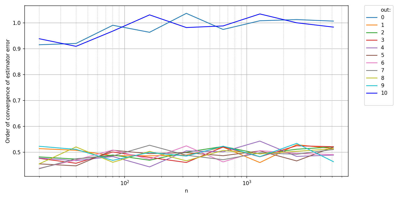
The above plot shows a very distinct behavior for the estimation of the minimum and maximum values compared to the other quantiles. The following plot of convergence order makes this difference even more salient.

pyquickbench.plot_benchmark(
    all_errors                      ,
    all_sizes                       ,
    all_funs                        ,
    plot_intent = plot_intent       ,
    show = True                     ,
    transform = "pol_cvgence_order" ,
    ylabel = "Order of convergence of estimator error"      ,
)