Time-consuming benchmarks

Benchmarking functions can be quite time consuming. This especially shows when the relative execution times of the different functions in the benchmark vary greatly. This is the case for the following general dense matrix-matrix multiplication benchmark:

import numpy as np
import numba as nb

numba_opt_dict = {
    'nopython':True     ,
    'cache':True        ,
    'fastmath':True     ,
    'nogil':True        ,
}

import pyquickbench

def python(a, b, c):

    for i in range(a.shape[0]):
        for j in range(b.shape[1]):
            for k in range(a.shape[1]):

                c[i,j] += a[i,k]*b[k,j]

def hybrid(a, b, c):

    for i in range(a.shape[0]):
        for j in range(b.shape[1]):

            c[i,j] = np.dot(a[i,:],b[:,j])

def numpy(a, b, c):
    np.matmul(a, b, out=c)

numba_serial = nb.jit(python,**numba_opt_dict)
numba_serial.__name__ = "numba_serial"

@nb.jit(parallel=True,**numba_opt_dict)
def numba_parallel(a, b, c):

    for i in nb.prange(a.shape[0]):
        for j in range(b.shape[1]):
            for k in range(a.shape[1]):

                c[i,j] += a[i,k]*b[k,j]

dtypes_dict = {
    "float32" : np.float32,
    "float64" : np.float64,
}

def setup_abc(n, real_dtype):
    a = np.random.random((n,n)).astype(dtype=dtypes_dict[real_dtype])
    b = np.random.random((n,n)).astype(dtype=dtypes_dict[real_dtype])
    c = np.zeros((n,n),dtype=dtypes_dict[real_dtype])
    return {'a':a, 'b':b, 'c':c}

all_args = {
    "n" : [(2 ** k) for k in range(8)]     ,
    "real_dtype": ["float32", "float64"]   ,
}

all_funs = [
    python          ,
    hybrid          ,
    numpy           ,
    numba_serial    ,
    numba_parallel  ,
]

n_repeat = 10

all_values = pyquickbench.run_benchmark(
    all_args                        ,
    all_funs                        ,
    setup = setup_abc               ,
    n_repeat = n_repeat             ,
    filename = timings_filename     ,
)

plot_intent = {
    "n"         : "points"          ,
    "real_dtype": "curve_linestyle" ,
}

pyquickbench.plot_benchmark(
    all_values                      ,
    all_args                        ,
    all_funs                        ,
    plot_intent = plot_intent       ,
    show = True                     ,
)

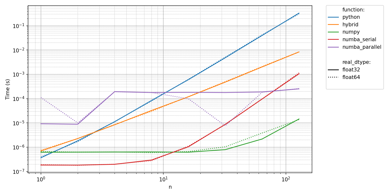
On the above plot, we can see that each call to the python implementation needs arround 0.1 s to complete, whereas the numpy implementation (backed up by BLAS’s dgemm) lasts less than a tenth of a milisecond. This is more than a 10 000 fold difference!

Even worse: the previous benchmark only explores the pre-asymptotic behavior of the numpy implementation, but running the benchmark with higher values of "n" would be extremely time consuming.

Since we know that typically, time measurements will be higher with higher values of "n", we can declare "n" as a MonotonicAxes. Pyquickbench will skip benchmarks for high values of the parameters declared in MonotonicAxes as soon as a certain timeout is reached. This allows much larger values to be explored at a reasonnable CPU cost.

basename = 'long_bench_2'
timings_filename = os.path.join(timings_folder, basename+'.npz')

MonotonicAxes = ["n"]
timeout = 10.        # Floating point value in seconds

all_args = {
    "n" : [(2 ** k) for k in range(15)]    ,
    "real_dtype": ["float32", "float64"]   ,
}

all_values = pyquickbench.run_benchmark(
    all_args                        ,
    all_funs                        ,
    setup = setup_abc               ,
    n_repeat = n_repeat             ,
    timeout = timeout               ,
    MonotonicAxes = MonotonicAxes   ,
    filename = timings_filename     ,
)

pyquickbench.plot_benchmark(
    all_values                      ,
    all_args                        ,
    all_funs                        ,
    plot_intent = plot_intent       ,
    show = True                     ,
)

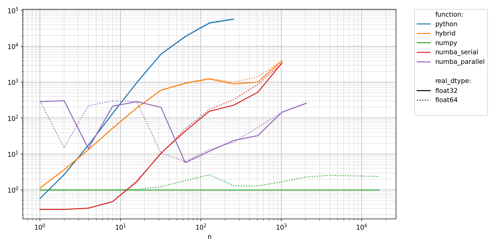
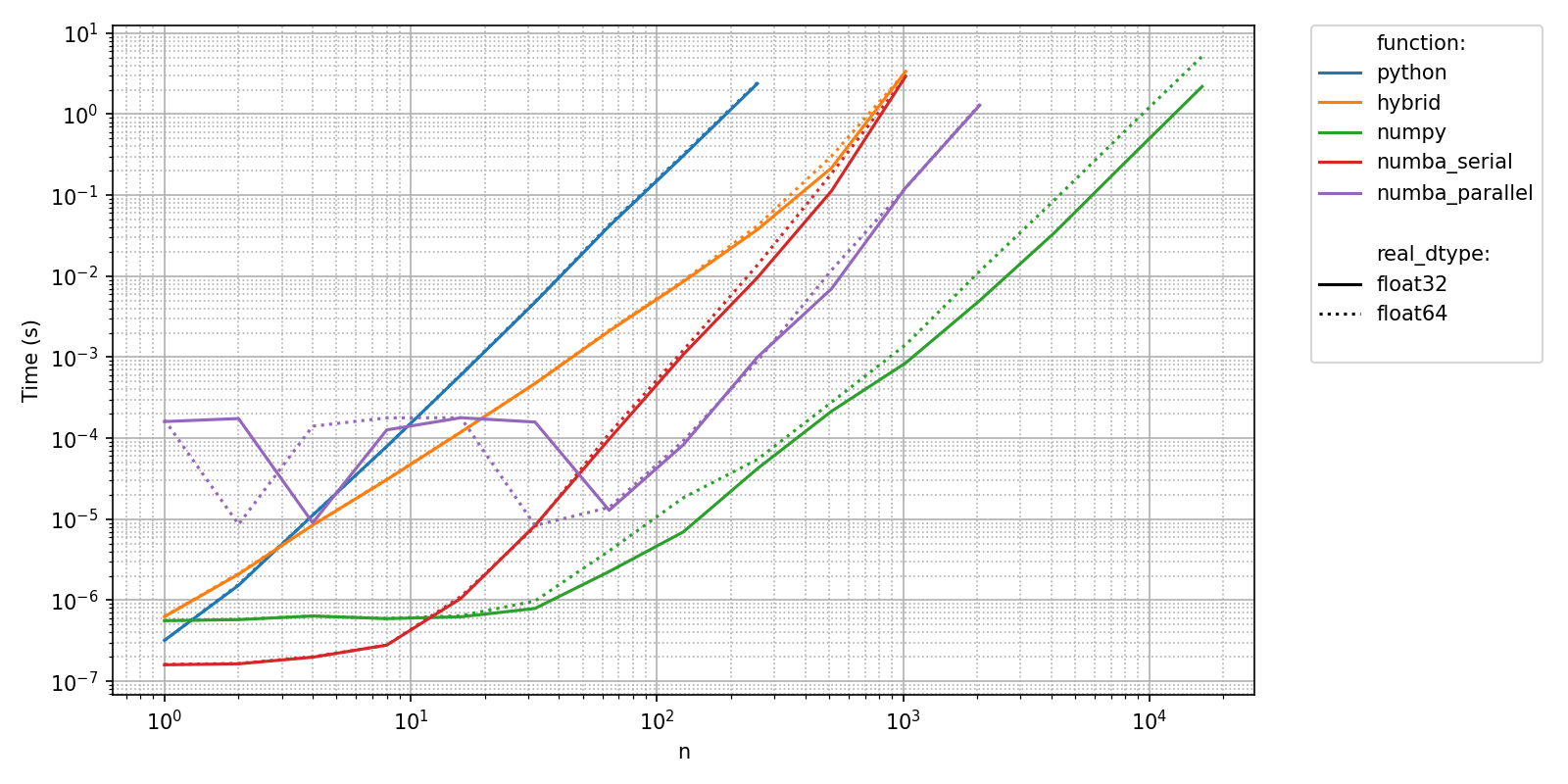
Plotting relative values shows that there can be a 100 000 fold difference between implementations!

relative_to_val = {
    "real_dtype": "float32"             ,
    pyquickbench.fun_ax_name : "numpy"  ,
}

pyquickbench.plot_benchmark(
    all_values                      ,
    all_args                        ,
    all_funs                        ,
    plot_intent = plot_intent       ,
    show = True                     ,
    relative_to_val = relative_to_val,
)

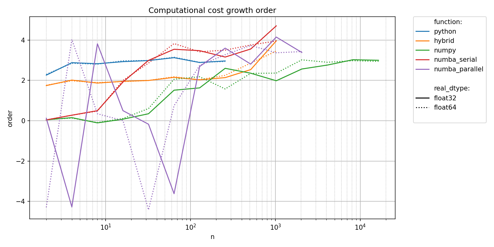
We can also see that different methods need different sizes of input to reach their theoretically cubic asymptotic regime.

pyquickbench.plot_benchmark(
    all_values                      ,
    all_args                        ,
    all_funs                        ,
    plot_intent = plot_intent       ,
    show = True                     ,
    title = "Computational cost growth order"   ,
    transform = "pol_growth_order"              ,
)