Plotting scalar values

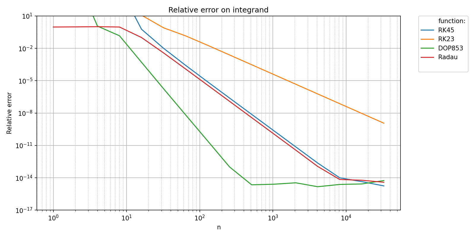
pyquickbench is not only designed to measure and plot the execution time of your Python routines, but also their output. Suppose you want to understand the convergence behavior of the following ODE integrators provided by scipy.integrate:

method_names = [
    "RK45"  ,
    "RK23"  ,
    "DOP853",
    "Radau" ,
]

Letting pyquickbench.run_benchmark() know that the benchmark target is the return value of the error function is as simple as passing mode = "scalar_output".

def scipy_ODE_cpte_error_on_test(
    method      ,
    n           ,
):

    # y'' = - w**2 * y
    # y(x) = A cos(w*x) + B sin(w*x)

    test_ndim = 2

    w = 10

    def ex_sol(t) :
        return np.array( [ np.cos(w*t) , np.sin(w*t),-np.sin(w*t), np.cos(w*t) ]  )

    def fgun(t, xy):

        fxy = np.empty(2*test_ndim)
        fxy[0] =  w*xy[2]
        fxy[1] =  w*xy[3]
        fxy[2] = -w*xy[0]
        fxy[3] = -w*xy[1]

        return fxy

    t_span = (0.,np.pi)

    max_step = (t_span[1] - t_span[0]) / n

    ex_init  = ex_sol(t_span[0])
    ex_final = ex_sol(t_span[1])

    bunch = scipy.integrate.solve_ivp(
        fun = fgun                      ,
        t_span = t_span                 ,
        y0 = ex_init                    ,
        method = method                 ,
        t_eval = np.array([t_span[1]])  ,
        first_step = max_step           ,
        max_step = max_step             ,
        atol = 1.                       ,
        rtol = 1.                       ,
    )

    error = np.linalg.norm(bunch.y[:,0]-ex_final)/np.linalg.norm(ex_final)

    return error

all_nint = np.array([2**i for i in range(16)])

bench = {
    method: functools.partial(
        scipy_ODE_cpte_error_on_test ,
        method  ,
    ) for method in method_names
}

plot_ylim = [1e-17, 1e1]

bench_filename = os.path.join(bench_folder,basename_bench_filename+'_error.npz')

pyquickbench.run_benchmark(
    all_nint                                    ,
    bench                                       ,
    mode = "scalar_output"                      ,
    filename = bench_filename                   ,
    plot_ylim = plot_ylim                       ,
    title = 'Relative error on integrand'       ,
    ylabel = "Relative error"                   ,
    show = True                                 ,
)

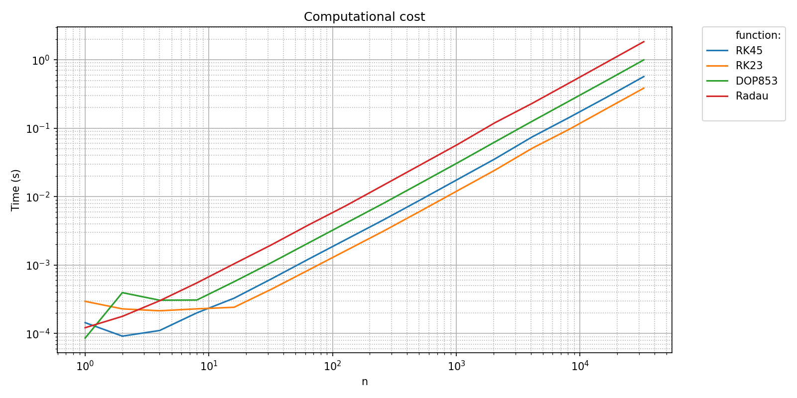
As seen in A first benchmark, the different integrations methods can be timed using pyquickbench with the following code, where we explicitely pass the default mode = "timings".

timings_filename = os.path.join(bench_folder,basename_bench_filename+'_timings.npz')

pyquickbench.run_benchmark(
    all_nint                        ,
    bench                           ,
    mode = "timings"                ,
    filename = timings_filename     ,
    logx_plot = True                ,
    title = 'Computational cost'    ,
    show = True                     ,
)

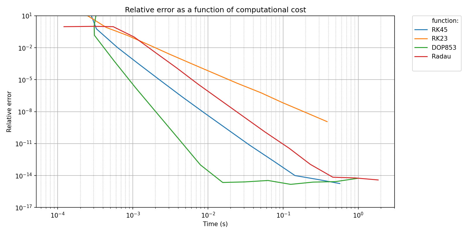
The best method for a given use case is a compromise between speed and accuracy. These two can be plotted against each other with the following code. Note that the benchmarks are not re-run thanks to the caching mechanism explained in Caching benchmarks.

bench_filename = os.path.join(bench_folder,basename_bench_filename+'_error.npz')

all_errors = pyquickbench.run_benchmark(
    all_nint                        ,
    bench                           ,
    mode = "scalar_output"          ,
    filename = bench_filename       ,
)

timings_filename = os.path.join(bench_folder,basename_bench_filename+'_timings.npz')

all_times = pyquickbench.run_benchmark(
    all_nint                        ,
    bench                           ,
    mode = "timings"                ,
    filename = timings_filename     ,
)

pyquickbench.plot_benchmark(
    all_errors                  ,
    all_nint                    ,
    bench                       ,
    mode = "scalar_output"      ,
    all_xvalues = all_times     ,
    logx_plot = True            ,
    plot_ylim = plot_ylim       ,
    title = 'Relative error as a function of computational cost' ,
    ylabel = "Relative error"   ,
    xlabel = "Time (s)"         ,
    show = True                 ,
)