Multidimensional benchmarks

One of pyquickbench’s strengths is its ability to run multidimensional benchmarks to test function behavior changes with respect to several different arguments, or to assess repeatability of a benchmark.

For instance, let’s run the following benchmark a thousand times.

import pyquickbench

def comprehension(n):
    return ['' for _ in range(n)]

def star_operator(n):
    return ['']*n

def for_loop_append(n):
    l = []
    for _ in range(n):
        l.append('')

all_funs = [
    comprehension   ,
    star_operator   ,
    for_loop_append ,
]

n_bench = 12
all_sizes = [2**n for n in range(n_bench)]

n_repeat = 1000
time_per_test = 0.2

all_values = pyquickbench.run_benchmark(
    all_sizes                       ,
    all_funs                        ,
    n_repeat = n_repeat             ,
    time_per_test = time_per_test   ,
    filename = timings_filename     ,
)

pyquickbench.plot_benchmark(
    all_values                      ,
    all_sizes                       ,
    all_funs                        ,
    show = True                     ,
)

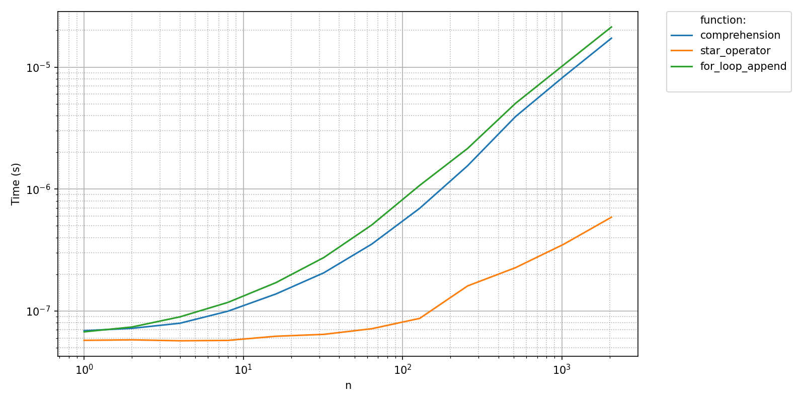
By default, only the minminum timing is reported on the plot as recommended by timeit.Timer.repeat(). This being said, the array all_values does contain n_repeat timings.

print(all_values.shape[0] == len(all_sizes))
print(all_values.shape[1] == len(all_funs))
print(all_values.shape[2] == n_repeat)

True
True
True

All the different timings can be superimposed on the same plot with the following plot_intent argument:

plot_intent = {
    pyquickbench.default_ax_name   : "points"       ,
    pyquickbench.fun_ax_name       : "curve_color"  ,
    pyquickbench.repeat_ax_name    : "same"         ,
}

pyquickbench.plot_benchmark(
    all_values                      ,
    all_sizes                       ,
    all_funs                        ,
    show = True                     ,
    plot_intent =   plot_intent     ,
)

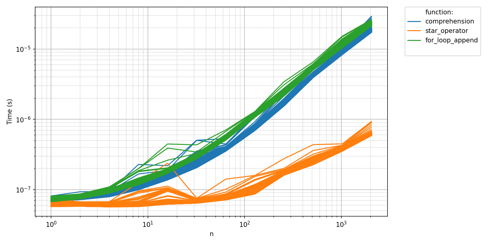
The above plot is quite cluttered. For more concise information, let’s use curve transparency:

pyquickbench.plot_benchmark(
    all_values                      ,
    all_sizes                       ,
    all_funs                        ,
    show = True                     ,
    plot_intent =   plot_intent     ,
    alpha = 1./255                  ,
)

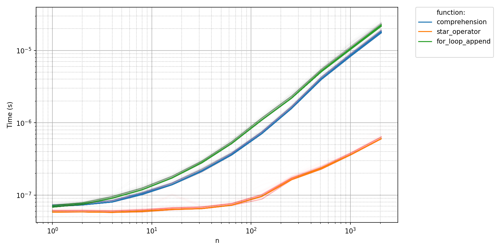
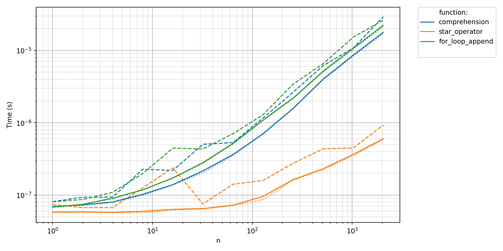
The above plot gives a good idea of the concentration of data, but bounds on timing are not very clear. Using reductions in plot_intent, we can for instance choose to plot minimal, median and maximal values. The list of all possible reductions is accessible in pyquickbench.all_reductions.

fig, ax = pyquickbench.plot_benchmark(
    all_values                  ,
    all_sizes                   ,
    all_funs                    ,
    return_empty_plot = True    ,
)

all_reductions = ["reduction_min", "reduction_max", "reduction_median"]
all_linestyles = ["dotted", "dashed", "solid"]

for (
    reduction   ,
    linestyle   ,
)in zip(
    all_reductions  ,
    all_linestyles  ,
):

    plot_intent = {
        pyquickbench.default_ax_name    : "points"      ,
        pyquickbench.fun_ax_name        : "curve_color" ,
        pyquickbench.repeat_ax_name     : reduction     ,
    }

    pyquickbench.plot_benchmark(
        all_values                  ,
        all_sizes                   ,
        all_funs                    ,
        plot_intent = plot_intent   ,
        linestyle_list = linestyle  ,
        fig = fig                   ,
        ax = ax                     ,
    )

plt.tight_layout()
plt.show()

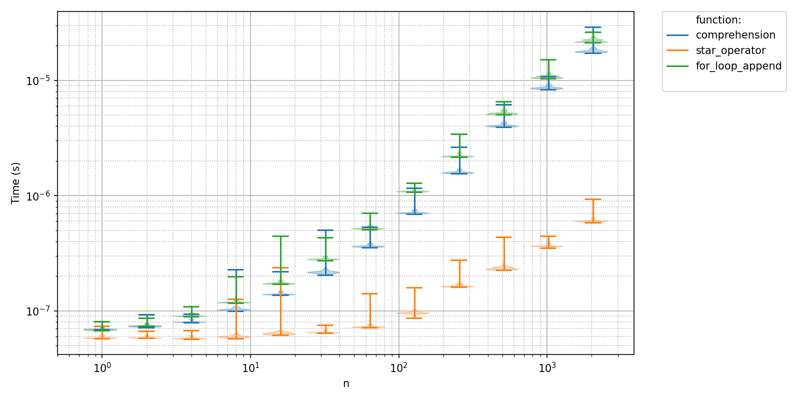
Another way to render data dispersion is to use the "violin" plot intent. This type of plot shows a Kernel Density Estimation of the timings distribution as well as extreme measured values for every set of input parameters.

plot_intent = {
    pyquickbench.default_ax_name    : "points"      ,
    pyquickbench.fun_ax_name        : "curve_color" ,
    pyquickbench.repeat_ax_name     : "violin"      ,
}

pyquickbench.plot_benchmark(
    all_values                  ,
    all_sizes                   ,
    all_funs                    ,
    plot_intent = plot_intent   ,
    show = True                 ,
)

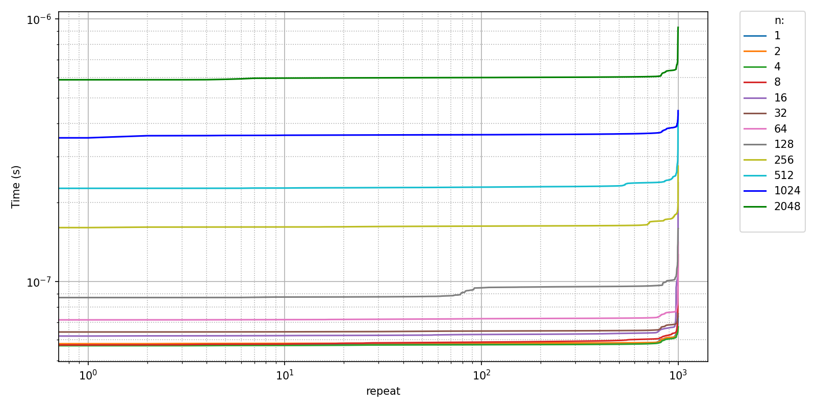
More generally, the plot_intent argument controls what dimension of the array all_values is plotted, and in what way. For instance, as a way to better understand the statistics of the measured timings, we can plot the measured time of execution as a function of the index of the repeated benchmark for a single function.

plot_intent = {
    pyquickbench.default_ax_name    : "curve_color"     ,
    pyquickbench.fun_ax_name        : "single_value"    ,
    pyquickbench.repeat_ax_name     : "points"          ,
}

single_values_val = {pyquickbench.fun_ax_name: "star_operator"}

pyquickbench.plot_benchmark(
    all_values                              ,
    all_sizes                               ,
    all_funs                                ,
    show = True                             ,
    plot_intent =   plot_intent             ,
    single_values_val = single_values_val   ,
)

Or for all functions, but a single value of input size.

plot_intent = {
    pyquickbench.default_ax_name    : "reduction_max"   ,
    pyquickbench.fun_ax_name        : "curve_color"     ,
    pyquickbench.repeat_ax_name     : "points"          ,
}

pyquickbench.plot_benchmark(
    all_values                      ,
    all_sizes                       ,
    all_funs                        ,
    show = True                     ,
    plot_intent = plot_intent       ,
)

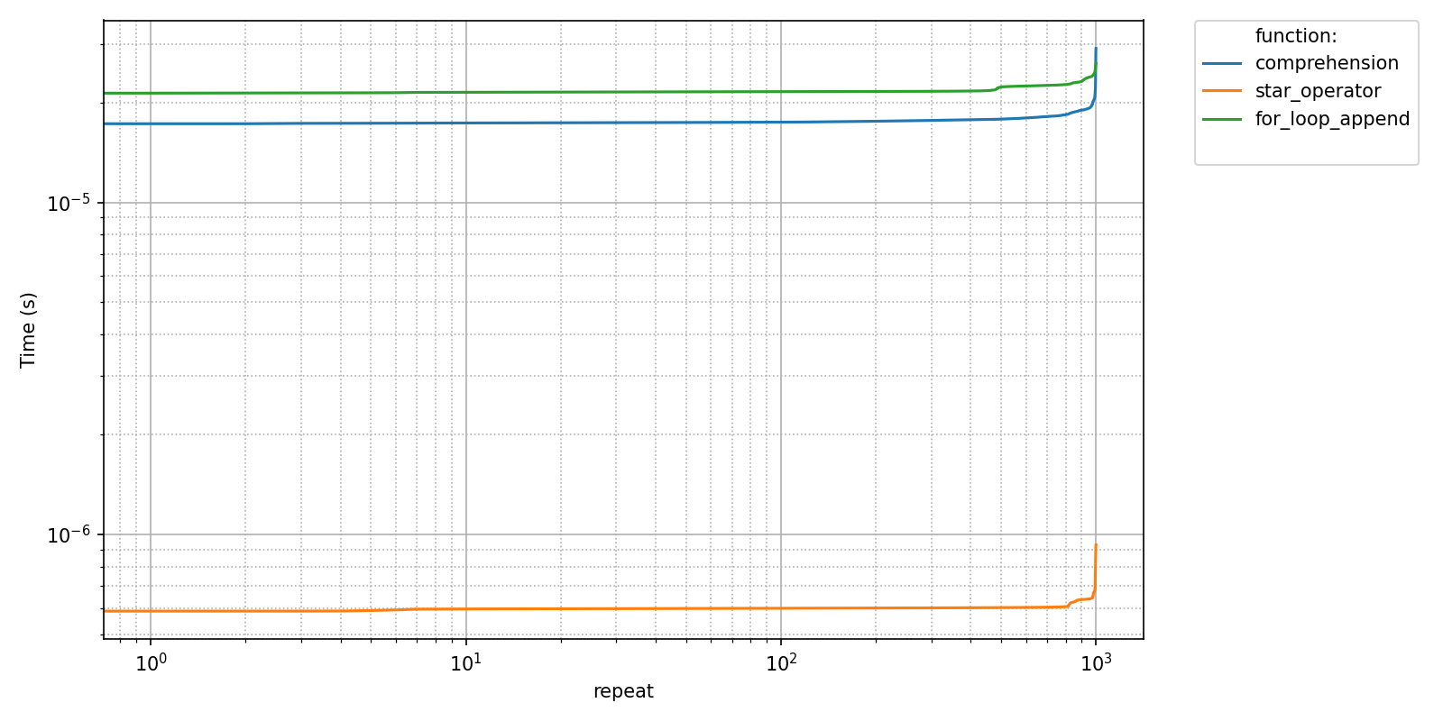
As can be seen in the above plots, the timings are automatically sorted along the pyquickbench.repeat_ax_name axis. The list of all possible plot_intent values is available in pyquickbench.all_plot_intents.