Convergence analysis of integration methods on segment

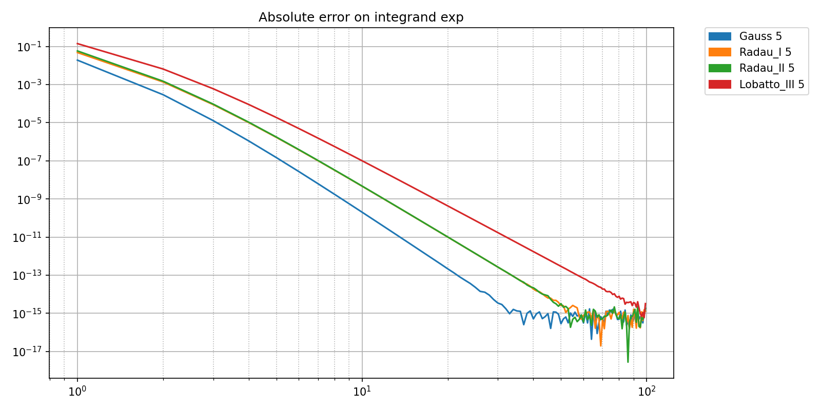
The following plots show the relative error made by different quadrature methods available as choreo.segm.quad.QuadTable on the integration of a smooth function (a scaled exponential).

all_integrands = [
    "exp",
]

methods = [
    'Gauss'         ,
    'Radau_I'       ,
    'Radau_II'      ,
    'Lobatto_III'   ,
    'Cheb_I'        ,
    'Cheb_II'       ,
    'ClenshawCurtis',
]

all_nsteps = [5,6]
refinement_lvl = np.array(range(1,100))

def setup(fun_name, quad_method, quad_nsteps, nint, DoEFT = False):
    return {'fun_name': fun_name, 'quad_method': quad_method, 'quad_nsteps': quad_nsteps, 'nint': nint, 'DoEFT':DoEFT}

all_args = {
    'integrand': all_integrands ,
    'quad_method': methods      ,
    'quad_nsteps': all_nsteps   ,
    'nint': refinement_lvl      ,
}

all_funs = [choreo.segm.test.Quad_cpte_error_on_test]

bench_filename = os.path.join(bench_folder, 'quad_cvg_bench.npz')

all_errors = pyquickbench.run_benchmark(
    all_args                        ,
    all_funs                        ,
    setup = setup                   ,
    mode = "scalar_output"          ,
    filename = bench_filename       ,
    ForceBenchmark = ForceBenchmark ,
    StopOnExcept = True             ,
    pooltype = "process"            ,
)

plot_intent = {
    'integrand': "subplot_grid_x"       ,
    'quad_method': "curve_color"        ,
    'quad_nsteps': "subplot_grid_y"     ,
    'nint': "points"                    ,
    pyquickbench.fun_ax_name : "same"   ,
}

fig, ax = pyquickbench.plot_benchmark(
    all_errors                              ,
    all_args                                ,
    all_funs                                ,
    plot_intent = plot_intent               ,
    title = 'Relative error of quadrature'  ,
    ylabel = "Relative error"               ,
)

plot_xlim = ax[0,0].get_xlim()
fig.tight_layout()
fig.show()

The following plots give the measured convergence rate as a function of the number of quadrature subintervals. The dotted lines are theoretical convergence rates.

plot_ylim = [0,15]

fig, ax = pyquickbench.plot_benchmark(
    all_errors                              ,
    all_args                                ,
    all_funs                                ,
    transform = "pol_cvgence_order"         ,
    plot_xlim = plot_xlim                   ,
    plot_ylim = plot_ylim                   ,
    logx_plot = True                        ,
    clip_vals = True                        ,
    stop_after_first_clip = True            ,
    plot_intent = plot_intent               ,
    title = 'Approximate convergence rate'  ,
)

for iy, nstep in enumerate(all_nsteps):
    for method in methods:

        quad = choreo.segm.multiprec_tables.ComputeQuadrature(nstep, method=method)
        th_order = quad.th_cvg_rate
        xlim = ax[iy,0].get_xlim()

        ax[iy,0].plot(xlim, [th_order, th_order], linestyle='dotted')

fig.tight_layout()
fig.show()

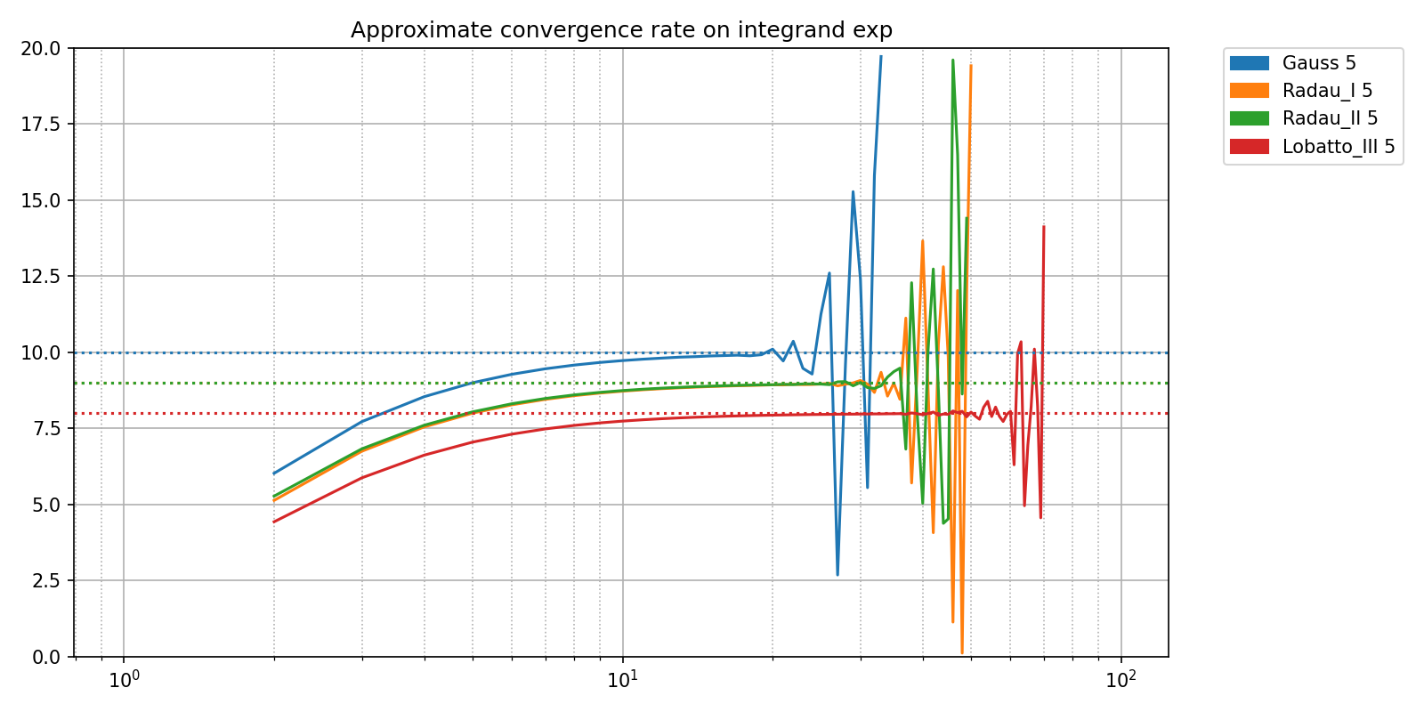
We can see 3 distinct phases on these plots:

• A first pre-convergence phase, where the convergence rate is growing towards its theoretical value. the end of the pre-convergence phase occurs for a number of sub-intervals roughtly independent of the convergence order of the quadrature method.

• A steady convergence phase where the convergence remains close to the theoretical value

• A final phase, where the relative error stagnates arround 1e-15. The value of the integral is computed with maximal accuracy given floating point precision. The approximation of the convergence rate is dominated by seemingly random floating point errors.

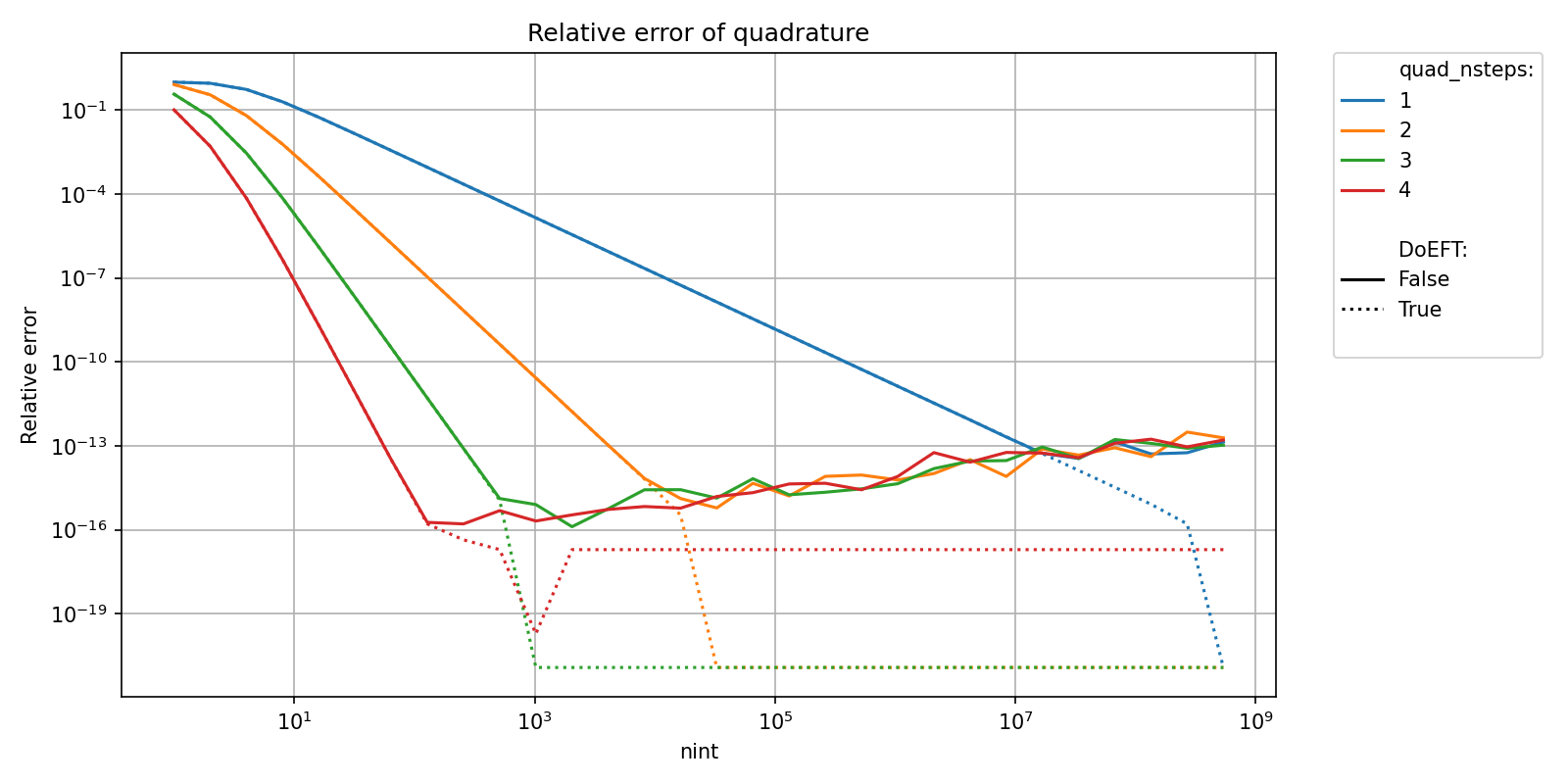
Now, if the number of integration steps is increased beyond what is necessary, these floating points error will start to steadily grow. This effect can be mitigated using a compensated summation algorithm. This is enabled by setting the argument DoEFT = True as shown below.

bench_filename = os.path.join(bench_folder,'quad_cvg_bench_EFT.npz')

refinement_lvl = np.array([2**n for n in range(30)])

all_args = {
    'integrand': all_integrands ,
    'quad_method': ['Gauss']    ,
    'quad_nsteps': [1, 2, 3, 4] ,
    'nint': refinement_lvl      ,
    'DoEFT': [False, True]      ,
}

plot_intent = {
    'integrand': "subplot_grid_x"       ,
    'quad_method': "subplot_grid_y"     ,
    'quad_nsteps': "curve_color"        ,
    'nint': "points"                    ,
    pyquickbench.fun_ax_name : "same"   ,
    'DoEFT' : "curve_linestyle"         ,
}

all_errors = pyquickbench.run_benchmark(
    all_args                        ,
    all_funs                        ,
    setup = setup                   ,
    mode = "scalar_output"          ,
    filename = bench_filename       ,
    ForceBenchmark = ForceBenchmark ,
    StopOnExcept = True             ,
    pooltype = "process"            ,
)

fig, ax = pyquickbench.plot_benchmark(
    all_errors                              ,
    all_args                                ,
    all_funs                                ,
    plot_intent = plot_intent               ,
    title = 'Relative error of quadrature'  ,
    ylabel = "Relative error"               ,

)