Note
Go to the end to download the full example code.
FFT and symmetries#
A few numerical investigation of how symmetries of a signal determine the shape of its discrete Fourier transform, and how to take advantage of this fact to optimize performance.
The spectral solvers in choreo make extensive use of the discrete Fourier transform to go back end forth between time representation (positions \(x_j = x(j/n)\)) and frequency representation (Fourier coefficients \(c_k\)) representation of orbits. Explicit formulae read:
The magic of FFT algorithms enables computation of all the positions from all the coefficients (and vice-versa) in \(\mathcal{O}(n\log(n))\) time instead of the naive \(\mathcal{O}(n^2)\).
Note that the total number of nodes needs to be divisible by 4 to properly account for symmetries
Real-valued signals and RFFT#
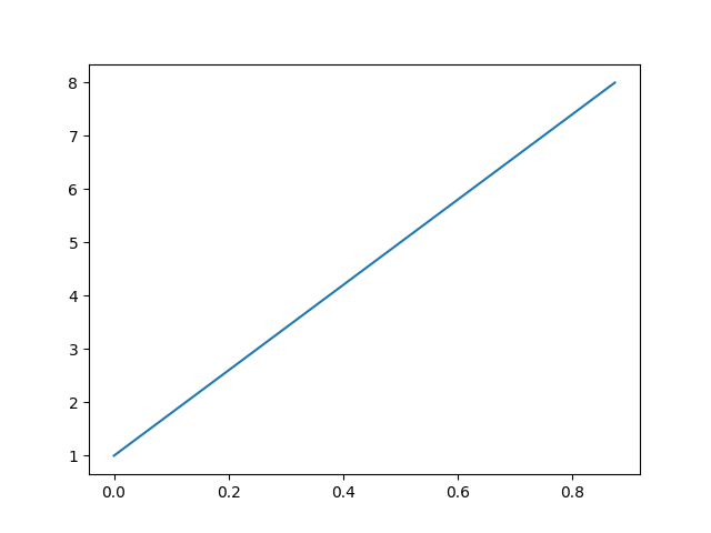
Signals we use in choreo are coordinates of the orbits, which are real-valued.
0.0
Therefore the FFT has Hermitian symmetry, meaning that the Fourier coefficients of negative index are the complex conjugates of their positive counterparts
0.0
This symmetry can be leveraged to only compute coefficients of positive index using the RFFT
rfft_c = scipy.fft.rfft(x)
err = np.linalg.norm(fft_c[:n//2+1] - rfft_c)
print(err)
0.0
The positions are retrieved using the IRFFT.
irfft_c = scipy.fft.irfft(rfft_c)
err = np.linalg.norm(irfft_c - x)
print(err)
0.0
Real-valued even signals and DCT I#
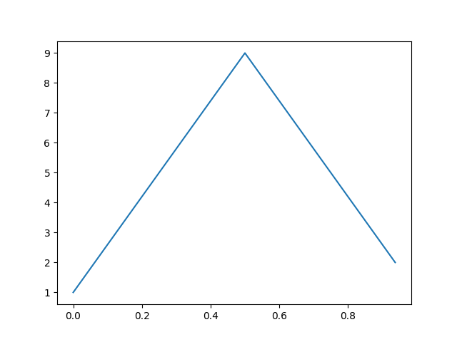
Suppose a coordinate of the orbit is constrained to be even.
n = 2*n_base   # Total number of nodes. Necessarily even here.
t = np.array(range(n))/n
y = np.array(range(n//2+1))+1
x = np.zeros(n)

for i in range(n//2+1):
    x[i] = y[i]

for i in range(n//2+1,n):
    x[i] = y[n - i]

z = np.zeros(n)
for i in range(n):
    z[i] = x[i] - x[(n-i) % n]

err = np.linalg.norm(z)
print(err)

plt.plot(t,x)
plt.show()
0.0
In this case, the Fourier transform is purely real, i.e. its imaginary part is zero.
rfft_c = scipy.fft.rfft(x)
err = np.linalg.norm(rfft_c.imag)
print(err)
8.881784197001252e-16
This symmetry can be leveraged to only compute the real part of the coefficients using the DCT I
dct_I_c = scipy.fft.dct(x[0:n//2+1],1)
err = np.linalg.norm(rfft_c.real - dct_I_c)
print(err)
0.0
Half the positions are retrieved using the IDCT I.
idct_I_x = scipy.fft.idct(dct_I_c,1)
err = np.linalg.norm(x[0:n//2+1] - idct_I_x)
print(err)
4.440892098500626e-16
Real-valued odd signals and DST I#
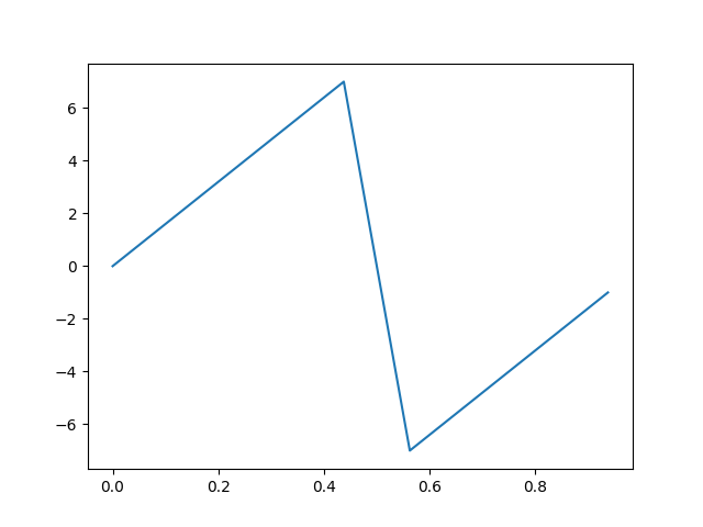
Suppose a coordinate of the orbit is constrained to be odd.
n = 2*n_base   # Total number of nodes. Necessarily even here.
t = np.array(range(n))/n
y = np.array(range(n//2-1))+1
x = np.zeros(n)

for i in range(1,n//2):
    x[i] = y[i-1]

for i in range(n//2+1,n):
    x[i] = - y[n - i - 1]

z = np.zeros(n)
for i in range(n):
    z[i] = x[i] + x[(n-i) % n]

err = np.linalg.norm(z)
print(err)

plt.plot(t,x)
plt.show()
0.0
In this case, the Fourier transform is purely imaginary, i.e. its real part is zero.
rfft_c = scipy.fft.rfft(x)
err = np.linalg.norm(rfft_c.real)
print(err)
1.7763568394002505e-15
This symmetry can be leveraged to only compute the imaginary part of the coefficients using the DST I
dst_I_c = scipy.fft.dst(x[1:n//2],1)
err = np.linalg.norm(rfft_c.imag[1:n//2] - (- dst_I_c))
print(err)
0.0
Half the positions are retrieved using the IDST I.
idst_I_x = scipy.fft.idst(dst_I_c,1)
err = np.linalg.norm(x[1:n//2] - idst_I_x)
print(err)
4.440892098500626e-16
Even - Odd decomposition of real-valued signals#
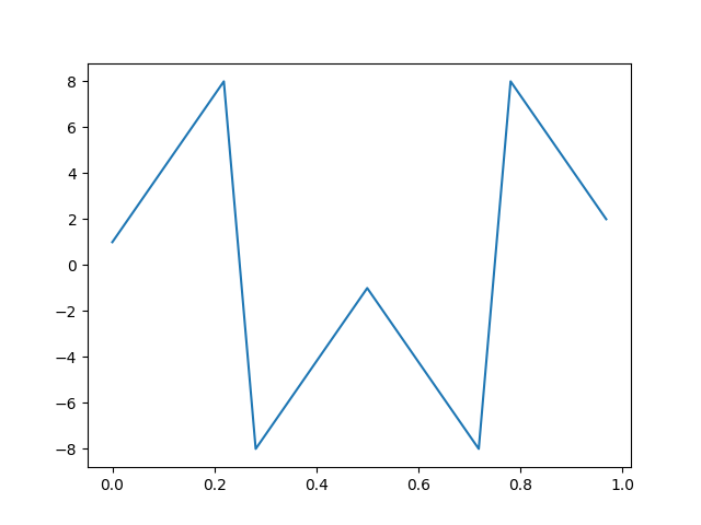
Any signal can be decomposed in even and odd parts
n = 2*n_base   # Total number of nodes. Necessarily even here.
t = np.array(range(n))/n
x = np.array(range(n))+1

x_even = np.zeros(n)
x_odd = np.zeros(n)
for i in range(n):
    x_even[i] = (x[i] + x[(n-i) % n]) / 2
    x_odd[i]  = (x[i] - x[(n-i) % n]) / 2


z = np.zeros(n)
for i in range(n):
    z[i] = x_even[i] - x_even[(n-i) % n]

err = np.linalg.norm(z)
print(err)

z = np.zeros(n)
for i in range(n):
    z[i] = x_odd[i] + x_odd[(n-i) % n]

err = np.linalg.norm(z)
print(err)

z = x - (x_even + x_odd)

err = np.linalg.norm(z)
print(err)

plt.plot(t,x)
plt.plot(t,x_even)
plt.plot(t,x_odd)
plt.show()
0.0
0.0
0.0
The even and odd parts can be transformed separately to form the transform of the initial signal
rfft_c = scipy.fft.rfft(x)
dct_I_c = scipy.fft.dct(x_even[0:n//2+1],1)
dst_I_c =  scipy.fft.dst(x_odd[1:n//2],1)

err = np.linalg.norm(rfft_c.real - dct_I_c)
print(err)
err = np.linalg.norm(rfft_c.imag[1:n//2] - (- dst_I_c))
print(err)
1.2560739669470201e-15
0.0
Real-valued even-odd signals and DCT III#
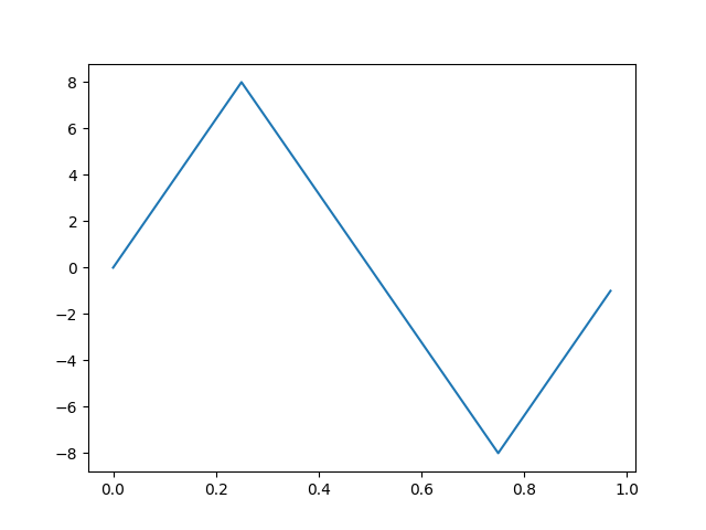
Suppose a coordinate of the orbit is constrained to be even arround the origin \(t=0\) and odd arround a quarter period \(t=T/4\).
n = 4*n_base   # Total number of nodes. Necessarily divisible by 4 here.
t = np.array(range(n))/n
y = np.array(range(n//4))+1
x = np.zeros(n)
for i in range(n//4):
    x[i] = y[i]

for i in range(n//4+1,n//2):
    x[i] = - y[n//2 - i]

for i in range(n//2,n//2 + n//4):
    x[i] = - y[i-n//2]

for i in range(n//2 + n//4 + 1,n):
    x[i] = y[n - i]

z = np.zeros(n)
for i in range(n):
    z[i] = x[i] - x[(n-i) % n]

err = np.linalg.norm(z)
print(err)

for i in range(n):
    z[i] = x[i] + x[(n+n//2 - i) % n]

err = np.linalg.norm(z)
print(err)


plt.plot(t,x)
plt.show()
0.0
0.0
In this case, the Fourier transform is purely real and its odd-numbered coefficients are zero.
rfft_c = scipy.fft.rfft(x)
err = np.linalg.norm(rfft_c.imag)
print(err)
err = np.linalg.norm(rfft_c[::2])
print(err)
8.51910812704787e-15
0.0
This symmetry can be leveraged to only compute the non-zero coefficients using the DCT III
dct_III_c = scipy.fft.dct(x[0:n//4],3)
err = np.linalg.norm(rfft_c.real[1::2] - 2*dct_III_c)
print(err)
6.646518689688359e-15
A quarter of the positions are retrieved using the IDCT III.
idct_III_c = scipy.fft.idct(dct_III_c,3)
err =  np.linalg.norm(x[0:n//4] - idct_III_c)
print(err)
1.831026719408895e-15
Real-valued odd-even signals and DST III#
Suppose a coordinate of the orbit is constrained to be odd arround the origin \(t=0\) and even arround a quarter period \(t=T/4\).
n = 4*n_base   # Total number of nodes. Necessarily divisible by 4 here.
t = np.array(range(n))/n
y = np.array(range(n//4))+1
x = np.zeros(n)

for i in range(1,n//4 + 1):
    x[i] = y[i-1]

for i in range(n//4+1,n//2):
    x[i] = y[n//2-1 - i]

for i in range(n//2+1,n//2 + n//4+1):
    x[i] = - y[i-(n//2+1)]

for i in range(n//2 + n//4+1,n):
    x[i] = -y[n-1 - i]

z = np.zeros(n)
for i in range(n):
    z[i] = x[i] + x[(n-i) % n]

err = np.linalg.norm(z)
print(err)

for i in range(n):
    z[i] = x[i] - x[(n+n//2 - i) % n]

err = np.linalg.norm(z)
print(err)

plt.plot(t,x)
plt.show()

0.0
0.0
In this case, the Fourier transform is purely imaginary and its even-numbered coefficients are zero.
rfft_c = scipy.fft.rfft(x)
err = np.linalg.norm(rfft_c.real)
print(err)
err = np.linalg.norm(rfft_c[::2])
print(err)
5.511875769711332e-15
0.0
This symmetry can be leveraged to only compute the non-zero coefficients using the DST III
dst_III_c = scipy.fft.dst(x[1:n//4+1],3)
err = np.linalg.norm(rfft_c.imag[1::2] - (-2*dst_III_c))
print(err)
9.532413939823706e-15
A quarter of the positions are retrieved using the IDCT III.
idst_III_c = scipy.fft.idst(dst_III_c,3)
err = np.linalg.norm(x[1:n//4+1] - idst_III_c)
print(err)
2.3914935841127266e-15
Real-valued signals with a subperiod#
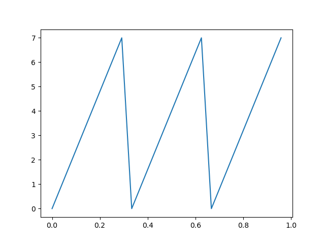
Suppose a coordinate of the orbit is constrained to have a period that is a multiple of the base period
sub_period = 3
n = n_base * sub_period # Total number of nodes. Necessarily a multiple of the sub period.
t = np.array(range(n))/n
y = np.array(range(n_base))
x = np.zeros(n)

for i in range(sub_period):
    for j in range(n_base):
        x[j+i*n_base] = y[j]

z = np.zeros(n)
for i_sub in range(sub_period-1):
    for i in range(n):
        z[i] = x[i] - x[(i+(i_sub+1)*n_base) % n]

    err = np.linalg.norm(z)
    print(err)

plt.plot(t,x)
plt.show()
0.0
0.0
In this case, the coefficients of the Fourier transform that are not indexed by a multiple of the subperiod are zero.
rfft_c = scipy.fft.rfft(x)
err = 0
for i in range(1,sub_period):
    err += np.linalg.norm(rfft_c[i::sub_period])

print(err)
0.0
This symmetry can be leveraged to only compute the non-zero coefficients using the RFFT on a sub-period only
rfftsub_c = scipy.fft.rfft(x[:n_base])
err = np.linalg.norm(rfft_c[::sub_period] - sub_period*rfftsub_c)
print(err)
6.4047456679787536e-15
The positions on a sub-period are retrieved using the RFFT.
irfftsub_c = scipy.fft.irfft(rfftsub_c)
err = np.linalg.norm(x[:n_base] - irfftsub_c)
print(err)
4.440892098500626e-16