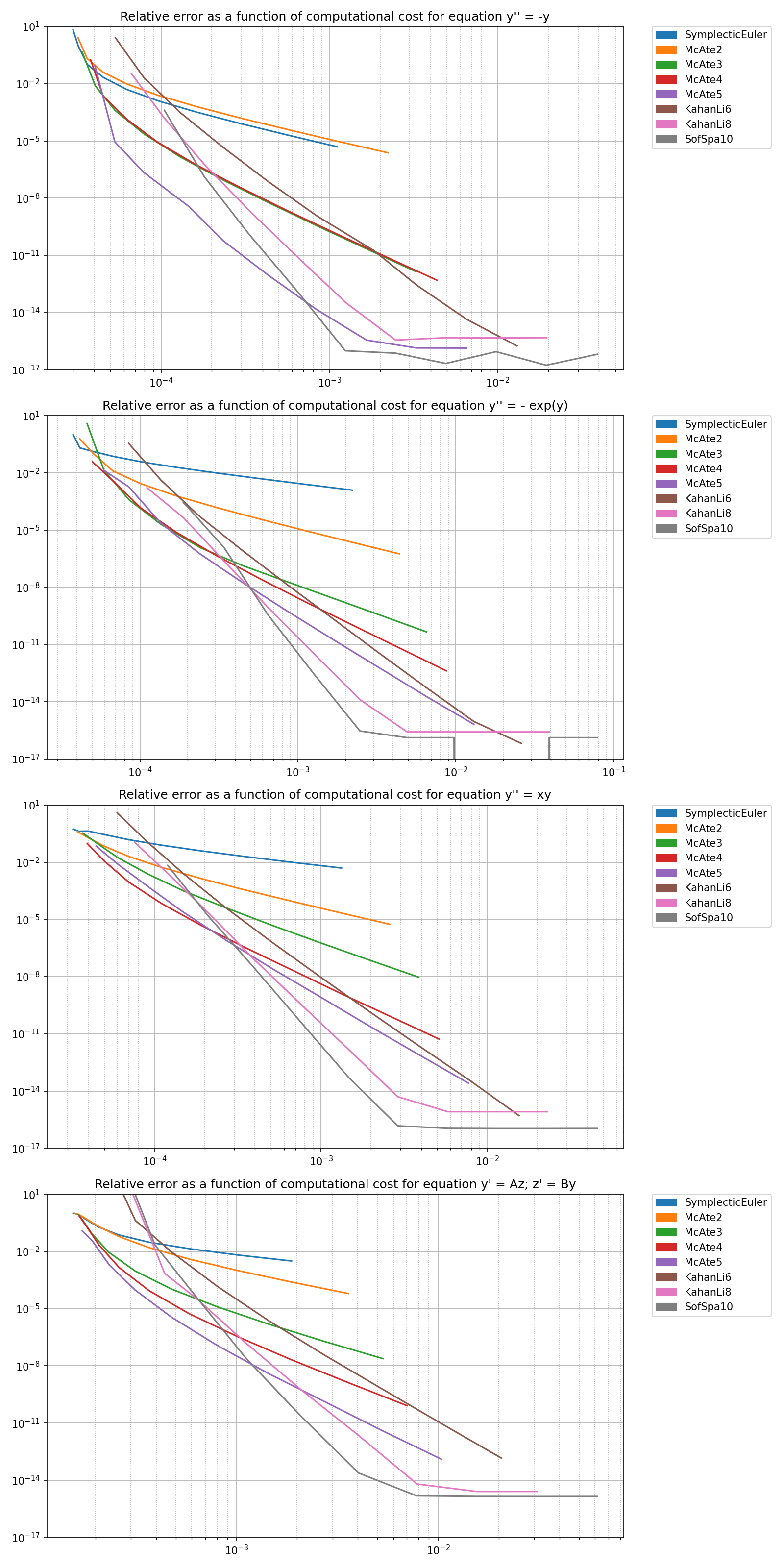
Convergence analysis of explicit Runge-Kutta methods for ODE IVP#

Evaluation of relative quadrature error with the following parameters:

eq_names = [
    "y'' = -y"          ,
    "y'' = - exp(y)"    ,
    "y'' = xy"          ,
    "y' = Az; z' = By"  ,
]


all_methods = { name : getattr(precomputed_tables,name) for name in dir(precomputed_tables) if isinstance(getattr(precomputed_tables,name),choreo.scipy_plus.ODE.ExplicitSymplecticRKTable) }

method_order_hierarchy = {}
for name, rk in all_methods.items():

    order = rk.th_cvg_rate

    cur_same_order = method_order_hierarchy.get(order, {})
    cur_same_order[name] = rk
    method_order_hierarchy[order] = cur_same_order

sorted_method_order = sorted(method_order_hierarchy)

The following plots give the measured relative error as a function of the number of quadrature subintervals

plt.show()

Relative error on integrand y'' = -y methods of order 1, Relative error on integrand y'' = - exp(y) methods of order 1, Relative error on integrand y'' = xy methods of order 1, Relative error on integrand y' = Az; z' = By methods of order 1, Relative error on integrand y'' = -y methods of order 2, Relative error on integrand y'' = - exp(y) methods of order 2, Relative error on integrand y'' = xy methods of order 2, Relative error on integrand y' = Az; z' = By methods of order 2, Relative error on integrand y'' = -y methods of order 3, Relative error on integrand y'' = - exp(y) methods of order 3, Relative error on integrand y'' = xy methods of order 3, Relative error on integrand y' = Az; z' = By methods of order 3, Relative error on integrand y'' = -y methods of order 4, Relative error on integrand y'' = - exp(y) methods of order 4, Relative error on integrand y'' = xy methods of order 4, Relative error on integrand y' = Az; z' = By methods of order 4, Relative error on integrand y'' = -y methods of order 5, Relative error on integrand y'' = - exp(y) methods of order 5, Relative error on integrand y'' = xy methods of order 5, Relative error on integrand y' = Az; z' = By methods of order 5, Relative error on integrand y'' = -y methods of order 6, Relative error on integrand y'' = - exp(y) methods of order 6, Relative error on integrand y'' = xy methods of order 6, Relative error on integrand y' = Az; z' = By methods of order 6, Relative error on integrand y'' = -y methods of order 8, Relative error on integrand y'' = - exp(y) methods of order 8, Relative error on integrand y'' = xy methods of order 8, Relative error on integrand y' = Az; z' = By methods of order 8, Relative error on integrand y'' = -y methods of order 10, Relative error on integrand y'' = - exp(y) methods of order 10, Relative error on integrand y'' = xy methods of order 10, Relative error on integrand y' = Az; z' = By methods of order 10

The following plots give the measured convergence rate as a function of the number of quadrature subintervals. The dotted lines are theoretical convergence rates.

plt.show()

Approximate convergence rate on integrand y'' = -y methods of order 1, Approximate convergence rate on integrand y'' = - exp(y) methods of order 1, Approximate convergence rate on integrand y'' = xy methods of order 1, Approximate convergence rate on integrand y' = Az; z' = By methods of order 1, Approximate convergence rate on integrand y'' = -y methods of order 2, Approximate convergence rate on integrand y'' = - exp(y) methods of order 2, Approximate convergence rate on integrand y'' = xy methods of order 2, Approximate convergence rate on integrand y' = Az; z' = By methods of order 2, Approximate convergence rate on integrand y'' = -y methods of order 3, Approximate convergence rate on integrand y'' = - exp(y) methods of order 3, Approximate convergence rate on integrand y'' = xy methods of order 3, Approximate convergence rate on integrand y' = Az; z' = By methods of order 3, Approximate convergence rate on integrand y'' = -y methods of order 4, Approximate convergence rate on integrand y'' = - exp(y) methods of order 4, Approximate convergence rate on integrand y'' = xy methods of order 4, Approximate convergence rate on integrand y' = Az; z' = By methods of order 4, Approximate convergence rate on integrand y'' = -y methods of order 5, Approximate convergence rate on integrand y'' = - exp(y) methods of order 5, Approximate convergence rate on integrand y'' = xy methods of order 5, Approximate convergence rate on integrand y' = Az; z' = By methods of order 5, Approximate convergence rate on integrand y'' = -y methods of order 6, Approximate convergence rate on integrand y'' = - exp(y) methods of order 6, Approximate convergence rate on integrand y'' = xy methods of order 6, Approximate convergence rate on integrand y' = Az; z' = By methods of order 6, Approximate convergence rate on integrand y'' = -y methods of order 8, Approximate convergence rate on integrand y'' = - exp(y) methods of order 8, Approximate convergence rate on integrand y'' = xy methods of order 8, Approximate convergence rate on integrand y' = Az; z' = By methods of order 8, Approximate convergence rate on integrand y'' = -y methods of order 10, Approximate convergence rate on integrand y'' = - exp(y) methods of order 10, Approximate convergence rate on integrand y'' = xy methods of order 10, Approximate convergence rate on integrand y' = Az; z' = By methods of order 10

We can see 3 distinct phases on these plots:

A first pre-convergence phase, where the convergence rate is growing towards its theoretical value. the end of the pre-convergence phase occurs for a number of sub-intervals roughtly independant of the convergence order of the quadrature method.
A steady convergence phase where the convergence remains close to the theoretical value
A final phase, where the relative error stagnates arround 1e-15. The value of the integral is computed with maximal accuracy given floating point precision. The approximation of the convergence rate is dominated by seemingly random floating point errors.

Error as a function of running time

plt.show()

Relative error as a function of computational cost for equation y'' = -y methods of order 1, Relative error as a function of computational cost for equation y'' = - exp(y) methods of order 1, Relative error as a function of computational cost for equation y'' = xy methods of order 1, Relative error as a function of computational cost for equation y' = Az; z' = By methods of order 1, Relative error as a function of computational cost for equation y'' = -y methods of order 2, Relative error as a function of computational cost for equation y'' = - exp(y) methods of order 2, Relative error as a function of computational cost for equation y'' = xy methods of order 2, Relative error as a function of computational cost for equation y' = Az; z' = By methods of order 2, Relative error as a function of computational cost for equation y'' = -y methods of order 3, Relative error as a function of computational cost for equation y'' = - exp(y) methods of order 3, Relative error as a function of computational cost for equation y'' = xy methods of order 3, Relative error as a function of computational cost for equation y' = Az; z' = By methods of order 3, Relative error as a function of computational cost for equation y'' = -y methods of order 4, Relative error as a function of computational cost for equation y'' = - exp(y) methods of order 4, Relative error as a function of computational cost for equation y'' = xy methods of order 4, Relative error as a function of computational cost for equation y' = Az; z' = By methods of order 4, Relative error as a function of computational cost for equation y'' = -y methods of order 5, Relative error as a function of computational cost for equation y'' = - exp(y) methods of order 5, Relative error as a function of computational cost for equation y'' = xy methods of order 5, Relative error as a function of computational cost for equation y' = Az; z' = By methods of order 5, Relative error as a function of computational cost for equation y'' = -y methods of order 6, Relative error as a function of computational cost for equation y'' = - exp(y) methods of order 6, Relative error as a function of computational cost for equation y'' = xy methods of order 6, Relative error as a function of computational cost for equation y' = Az; z' = By methods of order 6, Relative error as a function of computational cost for equation y'' = -y methods of order 8, Relative error as a function of computational cost for equation y'' = - exp(y) methods of order 8, Relative error as a function of computational cost for equation y'' = xy methods of order 8, Relative error as a function of computational cost for equation y' = Az; z' = By methods of order 8, Relative error as a function of computational cost for equation y'' = -y methods of order 10, Relative error as a function of computational cost for equation y'' = - exp(y) methods of order 10, Relative error as a function of computational cost for equation y'' = xy methods of order 10, Relative error as a function of computational cost for equation y' = Az; z' = By methods of order 10

Error as a function of running time for different orders

plt.show()

Relative error as a function of computational cost for equation y'' = -y, Relative error as a function of computational cost for equation y'' = - exp(y), Relative error as a function of computational cost for equation y'' = xy, Relative error as a function of computational cost for equation y' = Az; z' = By

Total running time of the script: (0 minutes 26.444 seconds)

Gallery generated by Sphinx-Gallery